Webscraping Sports Reference with R in 5 easy steps
How to use the rvest library to collect data for all your favorite sports
Up-to-date sports data can be found among the webpages of sportsreference.com for several of the worlds most popular sports, from college football to hockey, to baseball and soccer. This data, once accessed, can be used to build a variety of fascinating machine learning models to provide insights into performance analysis, scouting and draft projections, and game outcome prediction.
This tutorial explains how to webscrape data from a sports reference web page in 5 easy steps. Example code chunks for scraping college football rushing data are included with each step, with the full example code contained at end of this post.
1. Install and Load Rvest and Tidyverse packages
In order to scrape data from a web page in R, you will need to install and load the rvest package. Additionally, this tutorial uses a pipe operator to steamline the scraping process, which can be accessed by installing and loading the tidyverse library. If you already have the rvest and tidyverse packages installed, you do not need to install them again.
# install packages, as applicable
install.packages("rvest")
install.packages("tidyverse")

# load rvest and tidyverse libraries
library(rvest)
library(tidyverse)
A tutorial on webscraping in R without using the tidyverse can be found here.
For more information on the tidyverse, give tidyverse.org a visit.
2. Use Web Page URL to get HTML elements
After selecting a web page you want to scrape, save the url as a string object, and use the function read_html to read the html from the web page. You can also access the full html of a web page by using the command Ctrl + Shift + C (Command + Shift + C for Mac users) while in a web browser.
College Football example:
 my_url = "https://www.sports-reference.com/cfb/years/2021-rushing.html" # save url as R object

 read_html(my_url) # read html from my_url
3. Identify Web Page Characteristics and Scrape HTML Table(s)
Before applying rvest functionality further, it is important to understand the format of the web page which has the data you want to scrape. Specifically:
- Is the data already grouped into table elements?
- How many tables are there on the web page?
- Which table(s) on the web page do you want to scrape?
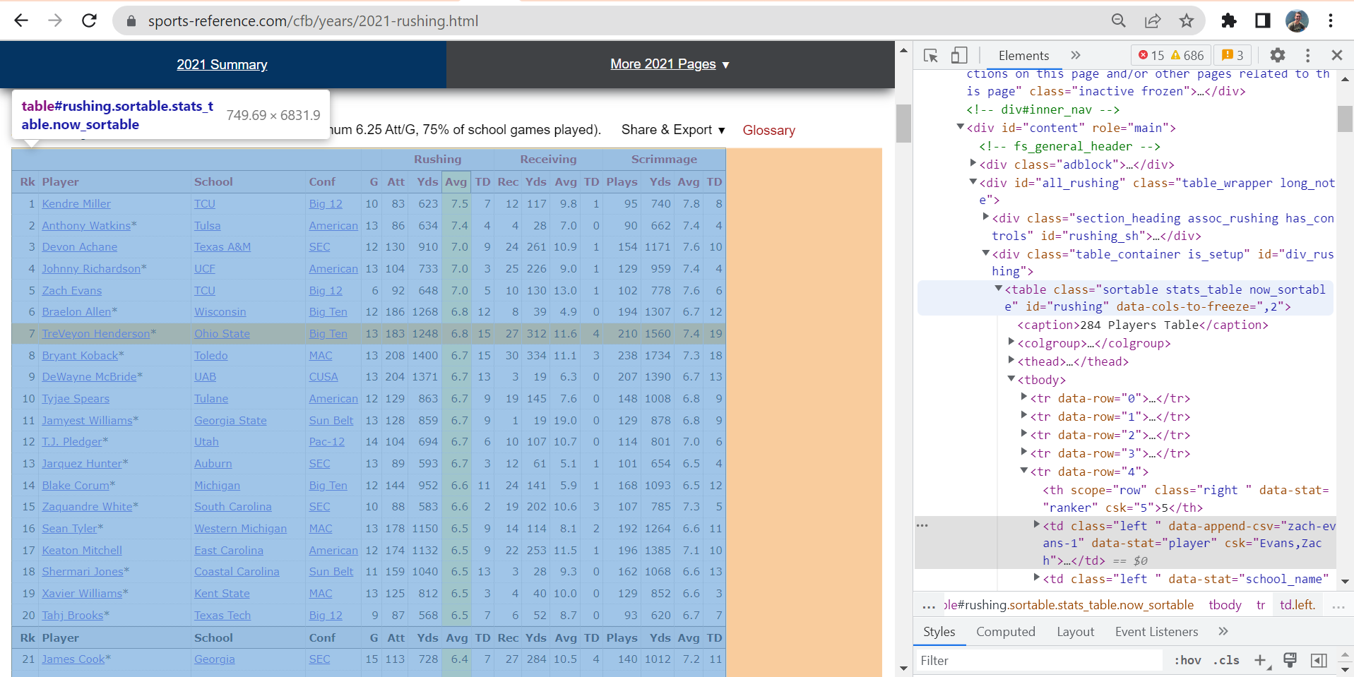
You can identify these characteristics with a quick scroll through of your web page, along with a right click + Inspect. This will open the HTML elements side bar, where you should look for for an element labeled <table>. For example, when inspecting the following College Football 2021 Rushing Stats web page, we can find the table element:
You can then scrape and store this data table by telling R to get the “table” html element from your read-in html, and then convert it into an R data frame. This can be done by simplying piping your read-in html into the functions html_element(), asking for the table element in quotation marks, then piping that into the html_table() function.
data_tbl <- read_html(url) %>% # read html from my_url
  html_element("table") %>% # get first table element
  html_table() # convert table to an R data frame (tibble)
Note: If a web page has more than one table, simply apply the html_elements() function in place of html_element(), which will import each of the desired tables as a list. You can then access your desired table by entering the index corresponding to the order of tables on the web page from top down.
 data_tbl <- read_html(my_url) %>%
  html_elements("table") %>% # get all table elements on web page and combine them into a list
  html_table() %>%
  .[[1]] # get first table
For a more in-depth description of web-page characteristics and HTML, see the opening sections of the dataquest article linked here: Tutorial: Web Scraping in R with rvest
4. Clean dataset header
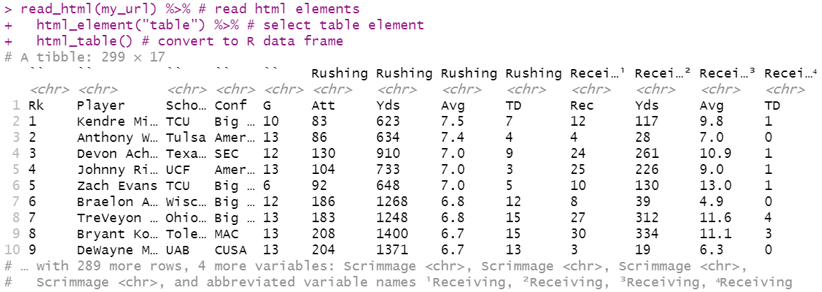
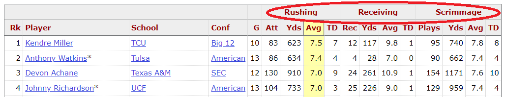
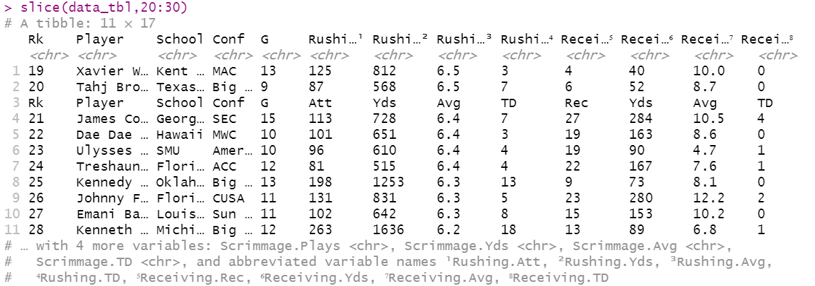
Two major issues often arise when scraping sports reference web pages, as shown in the screenshots below:
A) R confuses an extra header line as the true column names, and stores the true column names as the first row in the dataset.
B) Sports Reference pastes a reminder of the column names after every 20 rows in the dataset, which creates useless observations within the dataset.
These problems can be fixed in three simple lines of code:
1) Use the paste0() and colnames() functions to paste the current column names together with the current first row, and store this vector of names as the new table column names.
2) Use the gsub() and colnames() functions to find and replace any unecessary periods in the columns that did not have any informating in the extra header line (usually the first 5 columns).
3) Use the grepl() function in a slice of the data_tbl along with the ! “except” wildcard to only select observations that do not include header information. This can be found by searching for observations with the occurence of a column name in a given column, such as finding “Rk” in the Rk column.
# combine first row with second level of header above with period in between as new column names
colnames(data_tbl) = paste0(colnames(data_tbl), ".", data_tbl[1,]) # paste "original column name.value in first row" together as new column name

# remove periods from first few columns, which did not have a second, upper level heading
colnames(data_tbl)[1:5] = gsub("\\.", "", colnames(data_tbl[1:5]))  # find and replace all periods in first 5 columns with nothing (i.e., "")

# remove unneeded repeated header rows
data_tbl_clean = data_tbl[!grepl('Rk', data_tbl$Rk), ] # search for and do not include observations with "Rk" in the Rk column
5. Convert columns to correct data type to prepare for analysis
Lastly, due to the header issues presented in step 4, the web scraped data will likely incorrectly consider all variables as character variables. This can be amended by applying the as.numeric() function to relevant numeric columns using the sapply() function.
Note: For sports data, it will often be most efficient to apply as.numeric to all columns except those that should remain non-numeric, such as in the example below, which makes all columns numeric except for columns two through four.
# Prepare for analysis
data_tbl_clean[, -(2:4)]= sapply(data_tbl_clean[, -(2:4)], as.numeric) # ensure revelant continuous variables are interpreted as numeric variables
Conclusion
You now have the tools to get a plethora of sports data in practically the blink of eye with R. Now it’s your turn to try this out for yourself! Once you do, be sure to come back and comment what datasets you were able to create and what analysis you were able to perform with the skills outlined here and in other referenced sources.
Complete Code for Webscraping Sports Reference in R
# import libraries
library(tidyverse)
library(rvest)

# save url
my_url = "https://www.sports-reference.com/cfb/years/2021-rushing.html"

# webscraped tbl, saved as object
data_tbl <- read_html(my_url) %>% # read html elements
  html_element("table") %>% # select table element
  html_table() # convert to R data frame


# CLEAN TABLE
# take first row and combine with second level of header above with period in between words
colnames(data_tbl) = paste0(colnames(data_tbl), ".", data_tbl[1,])

# remove periods from first few columns
colnames(data_tbl)[1:5] = gsub("\\.", "", colnames(data_tbl[1:5]))

# remove unneeded repeated header rows
data_tbl_clean = data_tbl[!grepl('Rk', data_tbl$Rk), ]

# Prepare for analysis
data_tbl_clean[, -(2:4)]= sapply(data_tbl_clean[, -(2:4)], as.numeric) # ensure revelant continuous variables are interpreted as numeric variables

# cleaned, scraped data
data_tbl_clean
Acknowledgements
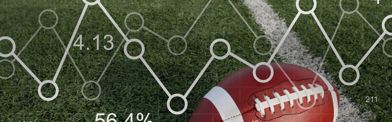
- Cover Image: The Athlytics Blog
- Complete rvest documentation: https://www.rdocumentation.org/packages/rvest/versions/1.0.3